Romain Francois, Professional R Enthusiast

To content | To menu | To search

Friday, July 3 2009

RGG#153: stars network

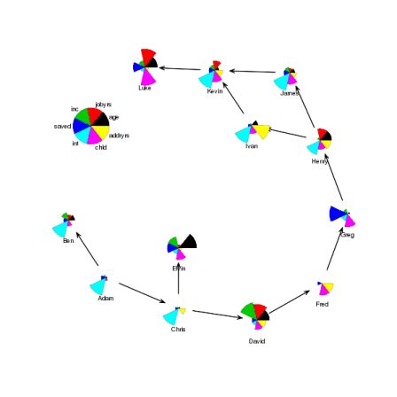
Graham Williams sent me this graph, now item 153 in the graph gallery.

graph_153.png

This plot draws a network but at the nodes we have simple segment plots (and in general we might have any other kind of plot at the nodes). This code constructs a network (from the network package), plots it with the nodes being invisibly plotted (using plot.network from the sna package) and then overlays the segment plots using the star function (with the key being located at a position determined by largest.empty from the Hmisc package.

Monday, June 22 2009

using ImageJ from R: the RImageJ package

I've pushed to CRAN the initial version of the RImageJ package. ImageJ is a java based image processing and analysis platform

This version of the package creates an instance of the IJ class as the IJ object in R, so that many methods of this class can be called using the dollar expansion of rJava.

Here is a simple example that uses the package:

download.file( "http://www.google.fr/intl/en_en/images/logo.gif", 
    dest = "google.gif" )

image = IJ$openImage( "google.gif" )
image$show()
IJ$run( "8-bit" )
IJ$run( "Invert" )
IJ$save( "bw-google.gif" )
image$close()


This downloads the google logo, convert it to black and white and inverts it

google logo bw-google.gif Future plans for this package contain:
  • integration of imagej and javagd
  • integration of the imagej macro recorder so that it creates R code instead of code in the imagej macro language

Wednesday, June 17 2009

with semantics for java objects in rJava

I've been playing with the rJava package recently. In a nutshell, rJava lets you create java objects and call methods on them from within the R console

col <- .jnew( "java/awt/Color", 255L, 0L, 0L )
.jcall( col, "I", "getRed" )
# [1] 255
col$getRed()
# [1] 255

The first call uses the regular function .jcall together with the JNI notation to call the getRed method of the created color, the second uses what rJava calls syntactic sugar, so that fields and methods of the object are accessed with the convenient R friendly dollar notation, great !!!

Here, I am just trying to add cream to make the coffee more tasty, by implementing the with method for java object

# This program is free software: you can redistribute it and/or modify
# it under the terms of the GNU General Public License as published by
# the Free Software Foundation, either version 2 of the License, or
# (at your option) any later version.
# 
# This program is distributed in the hope that it will be useful,
# but WITHOUT ANY WARRANTY; without even the implied warranty of
# MERCHANTABILITY or FITNESS FOR A PARTICULAR PURPOSE.  See the
# GNU General Public License for more details.
# 
# You should have received a copy of the GNU General Public License
# along with this program.  If not, see <http://www.gnu.org/licenses/>.

with.jobjRef <- function( data, expr, ...){
    
    env <- new.env( )
    clazz <- .jcall( data, "Ljava/lang/Class;", "getClass")
    fields <- .jcall( clazz, 
        "[Ljava/lang/reflect/Field;", "getFields" )
    lapply( fields, function(x ){
        n <- .jcall( x, "S", "getName" )
        makeActiveBinding( n, function(v){
            if( missing(v) ){
                # get 
                .jsimplify( .jcall( x, "Ljava/lang/Object;", "get", .jcast( data ) ) )
            } else {
                .jfield( data, n ) <- v
            }
        }, env ) 
    } )
    methods <- .jcall( clazz, 
        "[Ljava/lang/reflect/Method;", "getMethods" )
    lapply( methods, function(m){
        n <- .jcall( m, "S", "getName" )
        assign( n, function(...){
            .jrcall( data, n, ...) 
        }, env = env )
    } )
    assign( "this", data, env = env )
    eval( substitute( expr ), env = env )
}

This allows to call several methods on the same object, for example:

> with( col, {
+   cat( "red = ", getRed(), "\n" )
+   cat( "green = ", getGreen(), "\n" )
+   cat( "blue = ", getBlue(), "\n" )
+ })
red =  255 
green =  0 
blue =  0 
> p <- .jnew("java/awt/Point", 10L, 10L )
> with( p, {
+   move( 40L , 50L )
+   x <- y
+ } )
> p
[1] "Java-Object{java.awt.Point[x=50,y=50]}"

Note in the last example that the x variable that is assigned is the "x" field of the object

Tuesday, June 2 2009

Better completion popups

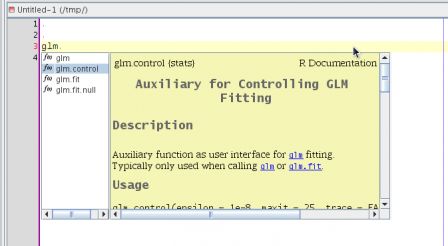
I've now updated the completion popups used in the advanced editor plugin to get a better display of the available information

For completion items that are related to functions with a help page, we now get this popup

completion-argument.png

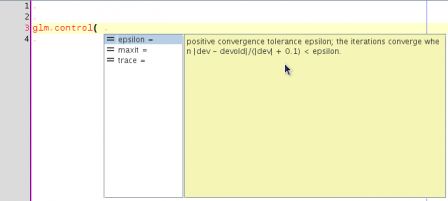
When completing arguments of functions, the text of the argument is grabbed from the help page (if available), and displayed as such:

completion-argument.png

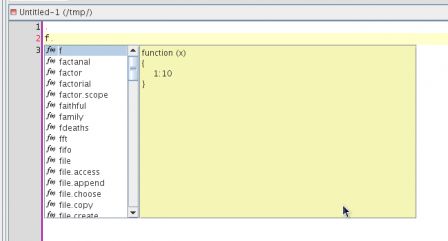
For functions that do not have help page, such as functions in the global environment, a deparse of the function is displayed

completion-argument.png

It is probably better to build the plugin from source, but otherwise I have posted a build here

I am currently working on ways to bring this completion mechanism to the console as well

Friday, May 29 2009

biocep's broken REPL

The REPL (Read Eval Print Loop) is the mechanism that R uses to (roughly):

  • get input from the console
  • send output to the console

JRI defines a mechanism for taking advantage of the REPL from java, through the RMainLoopCallbacks interface

biocep takes advantage of this infrastructure by implementing the interface within the DirectJNI class

To circumvent the fact that the REPL is basically an endless loop, gui front-ends usually let the loop run in its own thread, and set this thread to sleep whenever the user does something else than feeding the REPL. This is not quite the way it is done in biocep's implementation. In biocep, when there is no command to run, the REPL thread would wait a short amount of time and then send an empty string "" to the readConsole callback.

The reason why this is deficient is because R might not only use the REPL to ask for top-level command line commands, but also within the environment browser commonly used in R for debugging. Now feeding the browser prompt with an empty command has the effect of stepping out of it, making debugging impossible.

Here is patch against biocep that is a first attempt at solving this issue by implementing the REPL with a sleeping thread, inspired from the way the REPL is implemented in JGR. The patch has been made available to the author of biocep.

Thursday, May 28 2009

xterm256 support in biocep

On this post, I presented the xterm256 package for R, allowing to have text in background and foreground color in the R console

The drawback of relying on xterm escape sequences is that the package needs to be used within a terminal that supports this escape sequence protocol (basically some linux consoles)

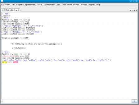
Here, I am proposing a patch to the biocep workbench that emulates support for these colors directly in the biocep R console, see the screenshot below:

xterm256-biocep.png

Combined with the syntax highlighter I am working on, this allows syntax highlighting of R code (pretty close to the way R sees the code) directly in the code and is in my view both visually pleasing and very useful

The functionality requires minor modifications of the source code of biocep that I have written and I can send a patch to interested users, but I unfortunately cannot commit the modifications to the biocep project because it is read-only at the moment

Wednesday, May 20 2009

Disable specific warnings

[This post is inspired from this thread on R-help]

The suppressWarnings function allows to call a function and suppress whatever warning it might generate. This uses the calling handler and restart mechanism of R to invoke the special "muffleWarning" restart when a warning is detected by the handler.

The downside is that it removes all warnings, and this might not be what you want. Consider that simple function that gives two warnings:

f <- function( x) {
  warning( "bla bla" )
  y <- x + 3
  warning( "yada yada" )
  y
}

> f(5)
[1] 8
Warning messages:
1: In f(5) : bla bla
2: In f(5) : yada yada
> suppressWarnings( f(5) )
[1] 8

What if I wanted to remove "bla bla" warnings and not "yada yada" warnings, because I know that "bla bla" warnings are expected and are more disturbing that useful. Currently, suppressWarnings does not offer that possibility, but you can make you own calling handler that handles warnings the way you want:

> h <- function(w) if( any( grepl( "bla", w) ) ) invokeRestart( "muffleWarning" )
> withCallingHandlers( f(5), warning = h )
[1] 8
Warning message:
In f(5) : yada yada

Thursday, May 7 2009

Search for R mailing list archives with gmane

This thread on R-devel led me to write these functions to search into R mailing list archives through gmane.
# This program is free software: you can redistribute it and/or modify
# it under the terms of the GNU General Public License as published by
# the Free Software Foundation, either version 3 of the License, or
# (at your option) any later version.
# 
# This program is distributed in the hope that it will be useful,
# but WITHOUT ANY WARRANTY; without even the implied warranty of
# MERCHANTABILITY or FITNESS FOR A PARTICULAR PURPOSE.  See the
# GNU General Public License for more details.
# 
# You should have received a copy of the GNU General Public License
# along with this program.  If not, see <http://www.gnu.org/licenses/>.

#' search on gmane.org mailing list archives
#'
#' @param string query
#' @param group search on which gmane group
#' @param author author of the email
#' @param sort sort order criteria
#' @param op how to combine words
#' @param r.group R related group to use, the default "*" means all r related groups
gmaneSearch <- function( string, 
    group = paste( "gmane.comp.lang.r.", r.group, sep = ""), 
    author = "", sort = c("relevance", "date", "revdate"), 
    op = c("and", "or"), 
    r.group = "*" ){
    
    sort <- match.arg(sort)
    op <- match.arg( op )
    
    url <- sprintf( 
        'http://search.gmane.org/?query=%s&author=%s&group=%s&sort=%s&DEFAULTOP=%s', 
            gsub( ' +', '+', string),  author,  group,  sort, op )
    url <- URLencode( url )
    browseURL( url )
}

#' retrieves the list of gmane groups associated with a prefix
#' 
#' @param prefix group prefix
gmaneGroups <- function( prefix = "gmane.comp.lang.r." ){
    url <- URLencode( sprintf( "http://dir.gmane.org/index.php?prefix=%s", prefix) )
    txt <- grep( '^<tr.*<td align=right.*<a', readLines( url ), value = TRUE )
    
    rx <- '^.*?<a href="(.*?)">(.*?)</a>.*<td>(.*?)</td>.*$'
    out <- data.frame( 
        url = gsub( rx, "\\1", txt ), 
        group = gsub( rx, "\\2", txt ),
        description = gsub( rx, "\\3", txt ), 
        stringsAsFactors = FALSE
        )
    out$group <- sub( "...", ".*", out$group, fixed = TRUE )
    out
}

So for example:

R> gmaneSearch ("browser prompt", author="romain" )
pops up this page

Saturday, April 18 2009

Colorful terminal: the R package "xterm256"

One of the goal of my forthcoming highlight package for R is to provide syntax highlighting based on evidence gathered from the output of the R parser directly into the R console (more on this later)

While writing the renderer targetting the console, I realized that support for colored text in the console is something that might be useful outside of the highlighter, and then decided to make it an independent package : xterm256

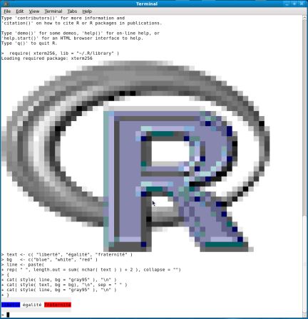
The idea is to use the The 256 color mode of xterm to wrap some text between escape sequences so that when it is cat to the console, the text appears with a background and/or a foreground color. Here is a screenshot from my console: lef-2.png

The package exposes only one function with three arguments: the style function with arguments :

  • x: the text we want to style
  • bg: the background color we want to use
  • fg: the foreground color we want to use

so if you want to print hello world in yellow with a black background, you can do:

cat( style( "hello world", bg = "black", fg = "yellow"), "\n" )

Friday, March 27 2009

Document java software with "R CMD build", ant, and javadoc

This is the sequel of this post where we look at ways to build javadoc documentation as part of an R package

Ant has the javadoc task which we will use to build html files from java sources, leading to this modified build script with the new javadoc target:

   1 <project name="Hello Java World" basedir="." default="build" >
   2 
   3   <property name="target.dir" value="../inst/java" />
   4   <property name="javadoc.dir" value="../inst/javadoc" />
   5   
   6   <target name="clean">
   7     <delete dir="bin" />
   8     <delete dir="${javadoc.dir}" />
   9   </target>
  10   
  11   <target name="compile">
  12     <mkdir dir="bin"/>
  13     <javac srcdir="src" destdir="bin" />
  14   </target>
  15   
  16   <target name="javadoc">
  17     <mkdir dir="${javadoc.dir}" />
  18     <javadoc access="public" destdir="${javadoc.dir}"
  19       author="true" version="true" use="true" 
  20       windowtitle="helloJavaWorld - Java API">
  21         
  22        <fileset dir="src" defaultexcludes="yes">
  23             <include name="**/*.java"/>
  24         </fileset>
  25           
  26     </javadoc>
  27   </target>
  28   
  29   <target name="build" depends="compile,javadoc">
  30     <jar jarfile="${target.dir}/hellojavaworld.jar">
  31       <fileset dir="bin" />
  32     </jar>
  33   </target>
  34   
  35 </project>
  36 

so that when we run "R CMD build", the directory inst/javadoc gets created and filled with documentation generated from the java sources

The next thing we need is a way to access this documentation from R documentation, so we will just add a link to it from the Rd file, I have added this into the helloJavaWorld.Rd file in the seealso section:

18 \seealso{\link[helloJavaWorld:../javadoc/index]{The Java API of the package}}

This is not a perfect solution but gives a starting point. Potential issues, things to improve :

  • It would be better to have a link in the 00Index.html file, but there currently is no way to do something like that
  • A way to jump back to the R documentation from the java documentation is needed

I have posted a copy of the built package here, and you can download the source of this version here

Next step, use the junitreport ant task to make a report of unit tests of the java code

Thursday, March 26 2009

Build java software with "R CMD build" and ant

The helloJavaWorld is a simple R package that shows how to distribute java software with an R package and communicate with it by means of the rJava package. helloJavaWorld has a vignette showing the different steps involved in making such a package.

Basically, helloJavaWorld uses the inst directory of an R package structure to ship the jar file in which the java software is packaged.

This post goes a bit further and shows how we can distribute the source of the java software and make R compile it when we run R CMD build. For that we are naturally going to use the src part of the R package, leading to this structure:

.
|-- DESCRIPTION
|-- NAMESPACE
|-- R
|   |-- helloJavaWorld.R
|   `-- onLoad.R
|-- inst
|   |-- doc
|   |   |-- helloJavaWorld.Rnw
|   |   |-- helloJavaWorld.pdf
|   |   `-- helloJavaWorld.tex
|   `-- java
|       `-- hellojavaworld.jar
|-- man
|   `-- helloJavaWorld.Rd
`-- src
    |-- Makevars
    |-- build.xml
    `-- src
        `-- HelloJavaWorld.java

7 directories, 12 files

Only the src directory differs from the version of helloJavaWorld that is on cran. Let's have a look at the files that are in src:

helloJavaWorld.java is the same as the code we can read in helloJavaWorld's vignette

   1 public class HelloJavaWorld {
   2    
   3   public String sayHello() {
   4     String result = new String("Hello Java World!");
   5     return result;
   6   }
   7 
   8   public static void main(String[] args) {
   9   }
  10 
  11 } 

build.xml is a simple ant script. Ant is typically used to build java software. This build script is very simple. It defines the following targets:

  • clean: removes the bin directory we use to store compiled class files
  • compile: compiles all java classes found in src into bin
  • build: package the java classes into the hellojavaworld.jar file, that we store in the inst/java directory to comply with the initial package structure
   1 <project name="Hello Java World" basedir="." default="build" >
   2 
   3   <property name="target.dir" value="../inst/java" />
   4   
   5   <target name="clean">
   6     <delete dir="bin" />
   7   </target>
   8   
   9   <target name="compile">
  10     <mkdir dir="bin"/>
  11     <javac srcdir="src" destdir="bin" />
  12   </target>
  13   
  14   <target name="build" depends="compile">
  15     <jar jarfile="${target.dir}/hellojavaworld.jar">
  16       <fileset dir="bin" />
  17     </jar>
  18   </target>
  19   
  20   
  21 </project>

Next, is the Makevars file. When an R package is built, R looks into the src directory for a Makevars file, which would typically be used to indicate how to compile the source code that is in the package. We simply use the Makevars file to launch the building and cleaning with ant, so we have a simple Makevars file:

   1 .PHONY: all
   2 
   3 clean:
   4     ant clean
   5 
   6 all: clean
   7     ant build
   8 

See Writing R extensions for details on the Makevars file

And now we can R CMD build the package:

$ R CMD build helloJavaWorld
* checking for file 'helloJavaWorld/DESCRIPTION' ... OK
* preparing 'helloJavaWorld':                          
* checking DESCRIPTION meta-information ... OK         
* cleaning src                                         
ant clean                                              
Buildfile: build.xml                                   

clean:

BUILD SUCCESSFUL
Total time: 0 seconds
* installing the package to re-build vignettes
* Installing *source* package ‘helloJavaWorld’ ...
** libs                                           
ant clean                                         
Buildfile: build.xml

clean:

BUILD SUCCESSFUL
Total time: 0 seconds
ant build
Buildfile: build.xml

compile:
    [mkdir] Created dir: /home/romain/svn/helloJavaWorld/src/bin
    [javac] Compiling 1 source file to /home/romain/svn/helloJavaWorld/src/bin

build:
      [jar] Building jar: /home/romain/svn/helloJavaWorld/inst/java/hellojavaworld.jar

BUILD SUCCESSFUL
Total time: 1 second
** R
** inst
** preparing package for lazy loading
** help
*** installing help indices
 >>> Building/Updating help pages for package 'helloJavaWorld'
     Formats: text html latex example
  helloJavaWorld                    text    html    latex   example
** building package indices ...
* DONE (helloJavaWorld)
* creating vignettes ... OK
* cleaning src
ant clean
Buildfile: build.xml

clean:
   [delete] Deleting directory /home/romain/svn/helloJavaWorld/src/bin

BUILD SUCCESSFUL
Total time: 0 seconds
* removing junk files
* checking for LF line-endings in source and make files
* checking for empty or unneeded directories
* building 'helloJavaWorld_0.0-7.tar.gz'

Download this version of helloJavaWorld: helloJavaWorld_0.0-7.tar.gz

This approach relies on ant being available, which we can specify in the SystemRequirements in the DESCRIPTION file

SystemRequirements: Java (>= 5.0), ant

Next time, we will see how to trick the documentation system so that it builds javadoc files

Monday, March 16 2009

A better jedit edit mode for R

I have spend a bit of time over the week end working with the jedit edit mode file for R code. That is the file that guides jedit on how to syntax highlight R code. The previous one I was using was based on the idea "let's put all the names of all the functions in standard R packages as keywords", although "it works", it is not a very good idea since it makes the edit mode huge and consequently must have some effect on jedit's performance when painting R code

The new mode file can be found on the biocep-editor project on r-forge

Here are some of the choices I have made

  • function calls are highlighted with type FUNCTION. A function call is a name followed by a round bracket
  • Core language constructs are highlighted with type KEYWORD1: (for, function, if, else, ifelse, in, repeat, return, switch, while, break, next) I have also added these to that list: (expression, quote, parse, deparse, substitute, get, getAnywhere, assign, exists, expression, bquote, typeof, mode, eval, evalq, with).
  • Debugging related functions are highlighted with type KEYWORD2: browser, debug, trace, traceback, recover, undebug, isdebugged, bp, mtrace
  • Error handling functions are highlighted using KEYWORD3: try, tryCatch, withRestarts, withCallingHandlers, stop, stopifnot, geterrmessage, warning, signalCondition, simpleCondition, simpleError, simpleWarning, simpleMessage, conditionCall, conditionMessage, computeRestarts, findRestart, invokeRestart, invokeRestartInteractively, isRestart, restartDescription, restartFormals, .signalSimpleWarning, .handleSimpleError
  • Object Oriented related functions (S3 and S4) are using type KEYWORD4: class, inherits, setClass, representation, structure, methods, setIs, slot, new, setMethod, validObject, setValidity, getValidity, initialize, setOldClass, callNextMethod, NextMethod, UseMethod, getS3method
  • Constants are using type LITERAL2: NULL, Inf, NULL, NA, NaN, T, TRUE, F, FALSE, pi, NA_character_, NA_complex_, NA_integer_, NA_real_
  • Apply functions are using LITERAL4: lapply, sapply, by, mapply, tapply, apply, replicate, aggregate. I have also added some functions from the packages reshape and plyr to that list
  • Support for R4X by delegating to the R4X mode (mainly XML) between strings "'##((xml" and "'##xml))"
  • Support for Roxygen comment, inspired from the way javadoc comments are treated in the java mode

Sunday, March 15 2009

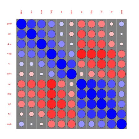
RGG#152: Correlation circles

For those out there looking for yet another way to represent a correlation matrix, Taiyun Wei has submitted the correlation circles graph_152.png

Tuesday, March 10 2009

Google Summer of Code idea

GSoC09.png

I've send today (right at the deadline point) an idea for a Google Summer of Code project to create an integrated debugger for R. The plan is to replace the tcltk front-end of the "debug" package with something giving a better user-experience. See the R Google Summer of Code page for details

Sunday, March 8 2009

Goldbach's Comet - take 2

Following this post, there is still room for improvement. Recall the last implementation (goldbach5)

12 goldbach5 <- function(n) {
13     xx <- 1 : n
14     xx <- xx[isprime(xx) > 0][-1]
15     
16     # generates row indices
17     x <- function(N){ 
18         rep.int( 1:N, N:1) 
19     }
20     # generates column indices
21     y <- function(N){ 
22         unlist( lapply( 1:N, seq.int, to = N ) ) 
23     }
24     z <- xx[ x(length(xx)) ] + xx[ y(length(xx)) ]
25     z <- z[z <= n]
26     tz <- tabulate(z, n )
27     tz[ tz != 0 ]
28 }
29 

The first thing to notice right away is that when we build xx in the first place, we are building integers from 1 to n, and check if they are prime afterwards. In that case, we are only going to need odd numbers in xx, so we can build them dircetly as:

31     xx <- seq.int( 3, n, by = 2)
32     xx <- xx[isprime(xx) > 0]

The next thing is that, even though the goldbach5 version only builds the upper triangle of the matrix, which saves some memory, we don't really need all the numbers, since eventually we just want to count how many times each of them appears. For that, there is no need to store them all in memory.

The version goldbach6 below takes this idea forward implementing the counting in C using the .C interface. See this section of writing R extensions for details of the .C interface.

30 goldbach6 <- function( n ){
31     xx <- seq.int( 3, n, by = 2)
32     xx <- xx[isprime(xx) > 0]
33     out <- integer( n )
34     tz <- .C( "goldbach", xx =as.integer(xx), nx = length(xx), 
35       out = out, n = as.integer(n), DUP=FALSE )$out
36     tz[ tz != 0 ]
37 }
38 

and the C function that goes with it

   1 #include <R.h>
   2  
   3 void goldbach(int * xx, int* nx, int* out, int* n){
   4     int i,j,k;
   5     
   6     for( i=0; i<*nx; i++){
   7         for( j=i; j<*nx; j++){
   8             k = xx[i] + xx[j] ;
   9             if( k > *n){
  10                 break;
  11             }
  12             out[k-1]++ ;
  13         }
  14     }
  15 }
  16 

We need to build the shared object

$ R CMD SHLIB goldbach.c
gcc -std=gnu99 -I/usr/local/lib/R/include  -I/usr/local/include    -fpic  -g -O2 -c goldbach.c -o goldbach.o
gcc -std=gnu99 -shared -L/usr/local/lib -o goldbach.so goldbach.o   -L/usr/local/lib/R/lib -lR

and load it in R:

> dyn.load( "goldbach.so" )

And now, let's see if it was worth the effort

> system.time( out <- goldbach6(100000) )
   user  system elapsed
  0.204   0.005   0.228
> system.time( out <- goldbach5(100000) )
   user  system elapsed
  4.839   2.630   7.981
> system.time( out <- goldbach4(100000) )
   user  system elapsed
 28.425   5.932  38.380

We could also have a look at the memoty footprint of each of the three functions using the memory profiler.

> gc(); Rprof( "goldbach4.out", memory.profiling=T ); out <- goldbach4(100000); Rprof(NULL) 
         used (Mb) gc trigger  (Mb)  max used   (Mb)                                        
Ncells 150096  4.1     350000   9.4    350000    9.4                                        
Vcells 213046  1.7  104145663 794.6 199361285 1521.1                                        
> gc(); Rprof( "goldbach5.out", memory.profiling=T ); out <- goldbach5(100000); Rprof(NULL) 
         used (Mb) gc trigger   (Mb)  max used   (Mb)                                       
Ncells 150093  4.1     350000    9.4    350000    9.4                                       
Vcells 213043  1.7  162727615 1241.6 199361285 1521.1                                       
> gc(); Rprof( "goldbach6.out", memory.profiling=T ); out <- goldbach6(100000); Rprof(NULL) 
         used (Mb) gc trigger  (Mb)  max used   (Mb)                                        
Ncells 150093  4.1     350000   9.4    350000    9.4                                        
Vcells 213043  1.7  130182091 993.3 199361285 1521.1  
> rbind( summaryRprof( filename="goldbach4.out", memory="both" )$by.total[1,] ,
+        summaryRprof( filename="goldbach5.out", memory="both" )$by.total[1,],
+        summaryRprof( filename="goldbach6.out", memory="both" )$by.total[1,] )
            total.time total.pct mem.total self.time self.pct
"goldbach4"      32.08       100     712.6      1.26      3.9
"goldbach5"       6.66       100     306.7      2.80     42.0
"goldbach6"       0.22       100       0.2      0.00      0.0

Saturday, March 7 2009

Goldbach's Comet

Murali Menon has posted on his blog code to calculate Goldbach partitions. Murali describes his approach to write the function, starting from brute force approach of loops, though the use of the Vectorize function, to some further optimized code using outer

This post is a follow up on Murali's attempt refining the extra mile

This is the last implementation on Murali's blog :

 1 goldbach4 <- function(n) {
 2     xx <- 1 : n
 3     xx <- xx[isprime(xx) > 0]
 4     xx <- xx[-1]
 5     z <- as.numeric(upperTriangle(outer(xx, xx, "+"), 
 6                     diag = TRUE))
 7     z <- z[z <= n]
 8     hist(z, plot = FALSE, 
 9          breaks = seq(4, max(z), by = 2))$counts
10 }
11 

As pointed out on the blog, although this is fast thanks to the clever vectorization of outer, there is some frustration of having to allocate a matrix of size N * N when you only need the upper triangle ( N*(N+1)/2 ). Furthermore, if we look in outer, we see that not only an N*N sized vector is created for the result (robj), but also for the vectors X and Y:

31         FUN <- match.fun(FUN)
32         Y <- rep(Y, rep.int(length(X), length(Y)))
33         if (length(X)) 
34             X <- rep(X, times = ceiling(length(Y)/length(X)))
35         robj <- FUN(X, Y, ...)
36         dim(robj) <- c(dX, dY)
37     }

This reminded me of the fun we had a few years ago with a similar problem. See the R wiki for a detailed optimization, and I am borrowing Tony Plate's idea for the goldbach5 approach here. The idea is basically to figure out the indices of the upper triangle part of the matrix before calculating it:

12 goldbach5 <- function(n) {
13     xx <- 1 : n
14     xx <- xx[isprime(xx) > 0]
15     xx <- xx[-1]
16     
17     # generates row indices
18     x <- function(N){ 
19         rep.int( 1:N, N:1) 
20     }
21     # generates column indices
22     y <- function(N){ 
23         unlist( lapply( 1:N, seq.int, to = N ) ) 
24     }
25     z <- xx[ x(length(xx)) ] + xx[ y(length(xx)) ]
26     z <- z[z <= n]
27     tz <- tabulate(z, n )
28     tz[ tz != 0 ]
29 }
30 

This gives a further boost to the execution time (only really visible with large n)

> system.time( out <- goldbach4(100000) )
   user  system elapsed
 28.268   5.389  36.347
>
> system.time( out <- goldbach5(100000) )
   user  system elapsed
  4.927   1.873   7.734

Let's take a look at the output from the profiler output for both functions

> Rprof( "goldbach5.out" ); out <- goldbach5(100000); Rprof( NULL)
> summaryRprof( "goldbach5.out" )$by.total
            total.time total.pct self.time self.pct
"goldbach5"       6.60     100.0      2.88     43.6
"<="              1.60      24.2      1.60     24.2
"+"               0.72      10.9      0.72     10.9
".C"              0.48       7.3      0.48      7.3
"unlist"          0.48       7.3      0.30      4.5
"tabulate"        0.48       7.3      0.00      0.0
"y"               0.48       7.3      0.00      0.0
"rep.int"         0.36       5.5      0.36      5.5
"x"               0.36       5.5      0.00      0.0
"lapply"          0.18       2.7      0.18      2.7
".Call"           0.08       1.2      0.08      1.2
"isprime"         0.08       1.2      0.00      0.0

> Rprof( "goldbach4.out" ); out <- goldbach4(100000); Rprof( NULL)
> summaryRprof( "goldbach4.out" )$by.total
                 total.time total.pct self.time self.pct
"goldbach4"           31.60     100.0      1.28      4.1
"upperTriangle"       23.56      74.6      2.10      6.6
"upper.tri"           12.48      39.5      0.00      0.0
"outer"                8.98      28.4      7.38     23.4
"col"                  5.96      18.9      5.96     18.9
"row"                  5.40      17.1      5.40     17.1
"hist.default"         5.24      16.6      0.86      2.7
"hist"                 5.24      16.6      0.00      0.0
".C"                   3.98      12.6      3.98     12.6
"<="                   2.02       6.4      2.02      6.4
"FUN"                  1.60       5.1      1.60      5.1
"as.numeric"           0.54       1.7      0.54      1.7
"max"                  0.22       0.7      0.22      0.7
"seq"                  0.22       0.7      0.00      0.0
"seq.default"          0.22       0.7      0.00      0.0
"is.finite"            0.16       0.5      0.16      0.5
".Call"                0.08       0.3      0.08      0.3
"isprime"              0.08       0.3      0.00      0.0
"sort.int"             0.02       0.1      0.02      0.1
""          0.02       0.1      0.00      0.0
"median.default"       0.02       0.1      0.00      0.0
"sort"                 0.02       0.1      0.00      0.0
"sort.default"         0.02       0.1      0.00      0.0

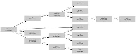
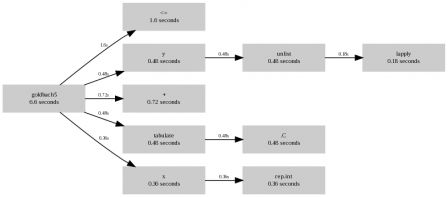
Or a graphical display (see the R wiki for the perl script that makes the graph):

goldbach4

goldbach4.png

goldbach5

goldbach5.png

The question is now, can we go further. I believe we can, because we still allocate a lot of things we trash eventually, any takers ?

What functions are called by my function

Quite often, it can be useful to identify which functions are being called by an R function. There are many ways to achieve this, such as for example massage the text representation of the function with regular expressions to basically find out what is just before round brackets.

The codetools package actually provides a much better way to do that, with the walkCode function.

# This program is free software: you can redistribute it and/or modify
# it under the terms of the GNU General Public License as published by
# the Free Software Foundation, either version 3 of the License, or
# (at your option) any later version.
# 
# This program is distributed in the hope that it will be useful,
# but WITHOUT ANY WARRANTY; without even the implied warranty of
# MERCHANTABILITY or FITNESS FOR A PARTICULAR PURPOSE.  See the
# GNU General Public License for more details.
# 
# You should have received a copy of the GNU General Public License
# along with this program.  If not, see .

#' Gets the functions called by fun
#' 
#' @param fun a function, or a character string
#' @return a named vector of occurences of each function, the values are 
#'         the number of times and the names are the functions
callees <- function( fun ){

    ## dump the function and read it back in the expression e
    # TODO: is there a better way
    #       If I just use body( fun ), I don't get the arguments
    fun <- match.fun( fun )
    con <- textConnection( NULL, open = "w" )
    dump( "fun", con )
    e <- parse( text = textConnectionValue(con) )[[1]]
    close( con )


    # initiate the functions vector whcih will be populated within
    # the code walker
    functions <- NULL
    env <- environment()

    # a code walker (see package codetools) that records function calls
    # this is inspired from the code walker used by showTree
    cw <- makeCodeWalker (
        call = function (e, w) {
            if( is.null(e) || length(e) == 0 ) return()

            # add the current function to the list
            env[["functions"]] <-
                    c( env[["functions"]], as.character(e[[1]]) )

            # process the list of expressions
            w$call.list( e[-1] , w )

        },
        leaf = function( e, w ){
            # deal with argument list of functions
            if( typeof( e ) == "pairlist" ){
                w$call.list( e, w )
            }
        },
        call.list = function( e, w ){
            for( a in as.list(e) ){
                if( !missing( a) ){
                    walkCode( a, w )
                }
            }
        },
        env = env # so that we can populate "functions"
    )

    # walk through the code with our code walker
    walkCode( e,  w = cw )

    # clean the output
    out <- table( functions )
    out[ order( names(out) ) ]

}
Let's try this on the jitter function:
> require( codetools )
> source("http://romainfrancois.blog.free.fr/public/posts/callees/callees.R")
> jitter
function (x, factor = 1, amount = NULL)
{
    if (length(x) == 0L)
        return(x)
    if (!is.numeric(x))
        stop("'x' must be numeric")
    z <- diff(r <- range(x[is.finite(x)]))
    if (z == 0)
        z <- abs(r[1L])
    if (z == 0)
        z <- 1
    if (is.null(amount)) {
        d <- diff(xx <- unique(sort.int(round(x, 3 - floor(log10(z))))))
        d <- if (length(d))
            min(d)
        else if (xx != 0)
            xx/10
        else z/10
        amount <- factor/5 * abs(d)
    }
    else if (amount == 0)
        amount <- factor * (z/50)
    x + stats::runif(length(x), -amount, amount)
}

> callees( jitter )
functions
        <-         ==          -         ::          !         !=          /
        10          4          2          1          1          1          4
         (          [          {          *          +        abs       diff
         1          2          2          2          1          2          2
     floor   function         if  is.finite    is.null is.numeric     length
         1          1          8          1          1          1          3
     log10        min      range     return      round      runif   sort.int
         1          1          1          1          1          1          1
     stats       stop     unique
         1          1          1

Tuesday, March 3 2009

Patching the R profiler so that it shows loops

The R profiler

The R profiler is an amazing way to find where in your code (or someone else's code) lies some inefficiency. For example, the profiler helped in this challenge on the R wiki. See also the profiling section on the http://cran.r-project.org/doc/manuals/R-exts.html#Profiling-R-code-for-speed document

What is wrong with it

The profiler, however, is not able to trace uses of loops (for, while or repeat), and consequently will not identify loops as the cause of ineffiency of the code. This is a shame, because loops in R are usually closely related to inefficiency. For example, if we profile this code:

1 Rprof( )
2 x <- numeric( )
3     for( i in 1:10000){
4       x <- c( x, rnorm(10) )
5     }
6 Rprof( NULL )
7 print( summaryRprof( ) )
8 
we get :
$ time Rscript script1.R 
$by.self
        self.time self.pct total.time total.pct
"rnorm"      0.16      100       0.16       100

$by.total
        total.time total.pct self.time self.pct
"rnorm"       0.16       100      0.16      100

$sampling.time
[1] 0.16


real	0m7.043s
user	0m5.170s
sys	0m0.675s

So the profiler only reports about 0.22 seconds, when the actual time taken is more about 5 seconds. We can show that by wrapping the entire for loop in a function:

   1 Rprof( )
   2 ffor <- function(){
   3     x <- numeric( )
   4     for( i in 1:10000){
   5       x <- c( x, rnorm(10) )
   6     }
   7 } 
   8 ffor()
   9 Rprof( NULL )
  10 print( summaryRprof( ) )
  11 

which gives this :

$ time Rscript script2.R 
$by.self
        self.time self.pct total.time total.pct
"ffor"       5.14     96.3       5.34     100.0
"rnorm"      0.20      3.7       0.20       3.7

$by.total
        total.time total.pct self.time self.pct
"ffor"        5.34     100.0      5.14     96.3
"rnorm"       0.20       3.7      0.20      3.7

$sampling.time
[1] 5.34


real	0m6.434s
user	0m5.151s
sys	0m0.698s

The ffor function takes 100 pourcent of the times, and rnorm takes only 3.7 percent of the time, instead of 100 percent, which would be the conclusion of the first example.

But in real life, it is not possible to wrap every loop in a function as this will massively break a lot of code. Instead, we could make the profiler aware of loops. This is the purpose of the patch I posted to R-devel

The details of the implementation

The patch actually only takes place in (several places of) the file eval.c

In the do_for function, a context is created for the "for" loop, using the begincontext function:

1033     begincontext(&cntxt, CTXT_LOOP, R_NilValue, rho, R_BaseEnv, R_NilValue,
1034          mkChar("[for]") );

The change here appears on the second line and simply adds a bit of information to the context that is created, similar changes are also made on the functions do_repeat and do_while.

Next, we need to grab this information at each tick of the profiler, which is the job of the doprof function:

168     if ((cptr->callflag & (CTXT_FUNCTION | CTXT_BUILTIN))
169         && TYPEOF(cptr->call) == LANGSXP) {
170         SEXP fun = CAR(cptr->call);
171         if (!newline) newline = 1;
172         fprintf(R_ProfileOutfile, "\"%s\" ",
173             TYPEOF(fun) == SYMSXP ? CHAR(PRINTNAME(fun)) :
174             "<Anonymous>");
175     } else if( (cptr->callflag & CTXT_LOOP) ){
176       if (!newline) newline = 1;
177       fprintf(R_ProfileOutfile, "\"%s\" ", CHAR(cptr->callfun) );  
178     }

The else branch will be executed when the context is a a loop context, and we just retrieve the callfun string we created in the do_for function.

Now, with this R patched, and compiled, Rprof is able to record loops

[]$ /home/romain/workspace/R-trunk/bin/Rscript script1.R
$by.self
        self.time self.pct total.time total.pct
"[for]"      5.28     97.4       5.42     100.0
"rnorm"      0.14      2.6       0.14       2.6

$by.total
        total.time total.pct self.time self.pct
"[for]"       5.42     100.0      5.28     97.4
"rnorm"       0.14       2.6      0.14      2.6

$sampling.time
[1] 5.42

[]$ head Rprof.out 
sample.interval=20000
"[for]" 
"[for]" 
"[for]" 
"rnorm" "[for]" 
"[for]" 
"[for]" 
"[for]" 
"[for]" 
"[for]" 
Friday, February 27 2009

Abstract submitted to useR! 2009

I've just submitted an abstract about the power editor at useR! 2009. The abstract is co-signed by Karim Chine (the author of biocep) who provided a lot of support during the development of the plugin and also written parts of it.

Last day to submit abstract to useR!

Today is the last day to submit an abstract to the next useR! conference and also to register online with the cheap rate.

- page 4 of 5 -