Romain Francois, Professional R Enthusiast

To content | To menu | To search

Tag - graphics

Entries feed - Comments feed

Friday, December 3 2010

Evolution of Rcpp code size


I've been contributing to Rcpp for about a year now, initially to add missing bits that were needed for the development of RProtoBuf. This led to a complete redesign of the API, which now goes way beyond the initial code (that we now call classic Rcpp API). This has been quite a journey in terms of development with more than 1500 commits to the svn repository of the project on R-forge, and promotion with presentations at RMetrics 2010, useR 2010, LondonR and at Google, as well as many blog posts about Rcpp and the packages that derive from it.

I wanted to take this opportunity to express visually how vibrant the development of Rcpp has been since it was first relaunched in 2008, and since I started to contribute.

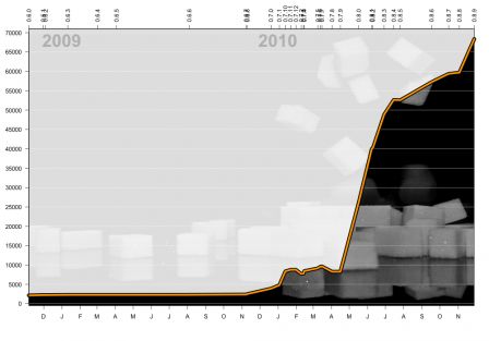
The graph below shows the evolution of the number of lines (counting the .h, .cpp, .R, .Rd, .Rnw files) accross released versions of the Rcpp package on CRAN

The first thing I need for this is to download the 32 versions of Rcpp that have been released since 0.6.0.

Then, all it takes is some processing with R to extract the relevant information (number of lines in files of interest), and present the data in a graph. I'm also taking this opportunity to have some fun with raster images and the png package
nlines_rcpp.png

The code explosion that started around version 0.7.8 marks the beginning of development of two of the most exciting and addictive projects I ever worked on: modules and sugar

The acceleration between 0.8.8 and the current version 0.8.9 represents many of the improvements that were made in modules. That alone, with more than 8000 new lines of code and documentation represents about 4 times as many lines as the total number of lines in 0.6.0

We still have plenty of ideas, and Rcpp will continue to evolve to deliver a quality interface between R and C++, to the best of the current team's abilities.

The full code is available below:
Tuesday, July 21 2009

RGG#155, 156 and 157

I pushed 3 more graphics from Biecek Przemyslaw to the graphics gallery

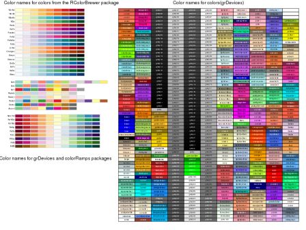
A list of popular names for colors from packages RColorBrewer, colorRamps, grDevices

graph_155.png

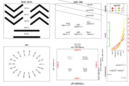
A set of examples of few graphical low-level parameters lend, ljoin, xpd, adj, legend(), axis, expressions, mtext, srt etc

graph_156.png

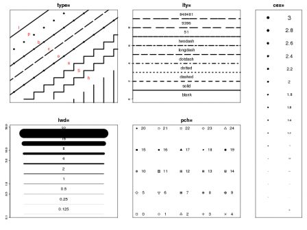
Examples for different settings of:

  • the type and width for lines
  • and the type and size for points

graph_157.png

Wednesday, July 8 2009

RGG# 154: demo of atomic functions

Przemyslaw Biecek has submitted this graph (and also others I will add later) to the graphics gallery

graph_154.png

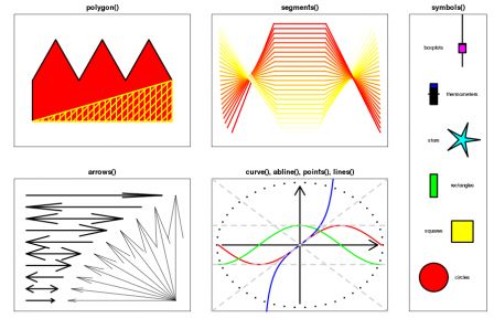
A list of examples for the atomic functions polygon(), segments(), symbols(), arrows(), curve(), abline(), points(), lines(). this figure is taken from the book Przewodnik po pakiecie R

Friday, July 3 2009

RGG#153: stars network

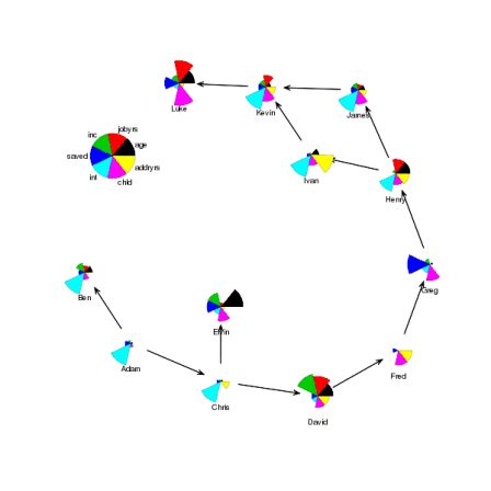
Graham Williams sent me this graph, now item 153 in the graph gallery.

graph_153.png

This plot draws a network but at the nodes we have simple segment plots (and in general we might have any other kind of plot at the nodes). This code constructs a network (from the network package), plots it with the nodes being invisibly plotted (using plot.network from the sna package) and then overlays the segment plots using the star function (with the key being located at a position determined by largest.empty from the Hmisc package.

Wednesday, February 4 2009

Graphic literacy improving? Let's try (RGG#150)

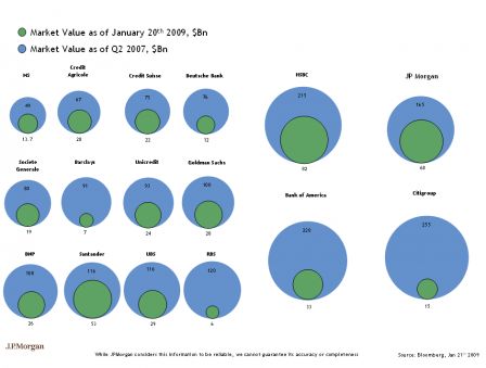
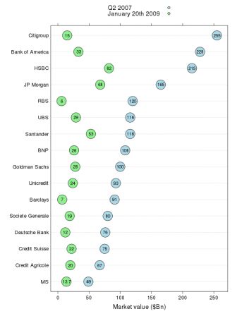
Here is a proposed alternative to this bubble inferno pointed out in the revolutions blog bubble.png ft.png and the R code behind it (here is the data). This is now item 150 in the graph gallery
   1 
   2 ### read the data
   3 d <- read.csv( "data.txt" )
   4 d$bank <- ordered( d$bank, levels = d$bank )
   5 
   6 ### load lattice and grid
   7 require( lattice )
   8 
   9 ### setup the key
  10 k <- simpleKey( c( "Q2 2007",  "January 20th 2009" ) )
  11 k$points$fill <- c("lightblue", "lightgreen")
  12 k$points$pch <- 21
  13 k$points$col <- "black"
  14 k$points$cex <- 1
  15 
  16 ### create the plot
  17 dotplot( bank ~ MV2007 + MV2009 , data = d, horiz = T, 
  18     par.settings = list( 
  19         superpose.symbol = list( 
  20             pch = 21, 
  21             fill = c( "lightblue", "lightgreen"), 
  22             cex = 4, 
  23             col = "black"  
  24         )
  25      ) , xlab = "Market value ($Bn)", key = k, 
  26      panel = function(x, y, ...){
  27        panel.dotplot( x, y, ... )
  28        grid.text( 
  29             unit( x, "native") , unit( y, "native") , 
  30             label = x, gp = gpar( cex = .7 ) )
  31      } )