Romain Francois, Professional R Enthusiast

To content | To menu | To search

Tag - profiling

Entries feed - Comments feed

Sunday, March 8 2009

Goldbach's Comet - take 2

Following this post, there is still room for improvement. Recall the last implementation (goldbach5)

12 goldbach5 <- function(n) {
13     xx <- 1 : n
14     xx <- xx[isprime(xx) > 0][-1]
15     
16     # generates row indices
17     x <- function(N){ 
18         rep.int( 1:N, N:1) 
19     }
20     # generates column indices
21     y <- function(N){ 
22         unlist( lapply( 1:N, seq.int, to = N ) ) 
23     }
24     z <- xx[ x(length(xx)) ] + xx[ y(length(xx)) ]
25     z <- z[z <= n]
26     tz <- tabulate(z, n )
27     tz[ tz != 0 ]
28 }
29 

The first thing to notice right away is that when we build xx in the first place, we are building integers from 1 to n, and check if they are prime afterwards. In that case, we are only going to need odd numbers in xx, so we can build them dircetly as:

31     xx <- seq.int( 3, n, by = 2)
32     xx <- xx[isprime(xx) > 0]

The next thing is that, even though the goldbach5 version only builds the upper triangle of the matrix, which saves some memory, we don't really need all the numbers, since eventually we just want to count how many times each of them appears. For that, there is no need to store them all in memory.

The version goldbach6 below takes this idea forward implementing the counting in C using the .C interface. See this section of writing R extensions for details of the .C interface.

30 goldbach6 <- function( n ){
31     xx <- seq.int( 3, n, by = 2)
32     xx <- xx[isprime(xx) > 0]
33     out <- integer( n )
34     tz <- .C( "goldbach", xx =as.integer(xx), nx = length(xx), 
35       out = out, n = as.integer(n), DUP=FALSE )$out
36     tz[ tz != 0 ]
37 }
38 

and the C function that goes with it

   1 #include <R.h>
   2  
   3 void goldbach(int * xx, int* nx, int* out, int* n){
   4     int i,j,k;
   5     
   6     for( i=0; i<*nx; i++){
   7         for( j=i; j<*nx; j++){
   8             k = xx[i] + xx[j] ;
   9             if( k > *n){
  10                 break;
  11             }
  12             out[k-1]++ ;
  13         }
  14     }
  15 }
  16 

We need to build the shared object

$ R CMD SHLIB goldbach.c
gcc -std=gnu99 -I/usr/local/lib/R/include  -I/usr/local/include    -fpic  -g -O2 -c goldbach.c -o goldbach.o
gcc -std=gnu99 -shared -L/usr/local/lib -o goldbach.so goldbach.o   -L/usr/local/lib/R/lib -lR

and load it in R:

> dyn.load( "goldbach.so" )

And now, let's see if it was worth the effort

> system.time( out <- goldbach6(100000) )
   user  system elapsed
  0.204   0.005   0.228
> system.time( out <- goldbach5(100000) )
   user  system elapsed
  4.839   2.630   7.981
> system.time( out <- goldbach4(100000) )
   user  system elapsed
 28.425   5.932  38.380

We could also have a look at the memoty footprint of each of the three functions using the memory profiler.

> gc(); Rprof( "goldbach4.out", memory.profiling=T ); out <- goldbach4(100000); Rprof(NULL) 
         used (Mb) gc trigger  (Mb)  max used   (Mb)                                        
Ncells 150096  4.1     350000   9.4    350000    9.4                                        
Vcells 213046  1.7  104145663 794.6 199361285 1521.1                                        
> gc(); Rprof( "goldbach5.out", memory.profiling=T ); out <- goldbach5(100000); Rprof(NULL) 
         used (Mb) gc trigger   (Mb)  max used   (Mb)                                       
Ncells 150093  4.1     350000    9.4    350000    9.4                                       
Vcells 213043  1.7  162727615 1241.6 199361285 1521.1                                       
> gc(); Rprof( "goldbach6.out", memory.profiling=T ); out <- goldbach6(100000); Rprof(NULL) 
         used (Mb) gc trigger  (Mb)  max used   (Mb)                                        
Ncells 150093  4.1     350000   9.4    350000    9.4                                        
Vcells 213043  1.7  130182091 993.3 199361285 1521.1  
> rbind( summaryRprof( filename="goldbach4.out", memory="both" )$by.total[1,] ,
+        summaryRprof( filename="goldbach5.out", memory="both" )$by.total[1,],
+        summaryRprof( filename="goldbach6.out", memory="both" )$by.total[1,] )
            total.time total.pct mem.total self.time self.pct
"goldbach4"      32.08       100     712.6      1.26      3.9
"goldbach5"       6.66       100     306.7      2.80     42.0
"goldbach6"       0.22       100       0.2      0.00      0.0
Saturday, March 7 2009

Goldbach's Comet

Murali Menon has posted on his blog code to calculate Goldbach partitions. Murali describes his approach to write the function, starting from brute force approach of loops, though the use of the Vectorize function, to some further optimized code using outer

This post is a follow up on Murali's attempt refining the extra mile

This is the last implementation on Murali's blog :

 1 goldbach4 <- function(n) {
 2     xx <- 1 : n
 3     xx <- xx[isprime(xx) > 0]
 4     xx <- xx[-1]
 5     z <- as.numeric(upperTriangle(outer(xx, xx, "+"), 
 6                     diag = TRUE))
 7     z <- z[z <= n]
 8     hist(z, plot = FALSE, 
 9          breaks = seq(4, max(z), by = 2))$counts
10 }
11 

As pointed out on the blog, although this is fast thanks to the clever vectorization of outer, there is some frustration of having to allocate a matrix of size N * N when you only need the upper triangle ( N*(N+1)/2 ). Furthermore, if we look in outer, we see that not only an N*N sized vector is created for the result (robj), but also for the vectors X and Y:

31         FUN <- match.fun(FUN)
32         Y <- rep(Y, rep.int(length(X), length(Y)))
33         if (length(X)) 
34             X <- rep(X, times = ceiling(length(Y)/length(X)))
35         robj <- FUN(X, Y, ...)
36         dim(robj) <- c(dX, dY)
37     }

This reminded me of the fun we had a few years ago with a similar problem. See the R wiki for a detailed optimization, and I am borrowing Tony Plate's idea for the goldbach5 approach here. The idea is basically to figure out the indices of the upper triangle part of the matrix before calculating it:

12 goldbach5 <- function(n) {
13     xx <- 1 : n
14     xx <- xx[isprime(xx) > 0]
15     xx <- xx[-1]
16     
17     # generates row indices
18     x <- function(N){ 
19         rep.int( 1:N, N:1) 
20     }
21     # generates column indices
22     y <- function(N){ 
23         unlist( lapply( 1:N, seq.int, to = N ) ) 
24     }
25     z <- xx[ x(length(xx)) ] + xx[ y(length(xx)) ]
26     z <- z[z <= n]
27     tz <- tabulate(z, n )
28     tz[ tz != 0 ]
29 }
30 

This gives a further boost to the execution time (only really visible with large n)

> system.time( out <- goldbach4(100000) )
   user  system elapsed
 28.268   5.389  36.347
>
> system.time( out <- goldbach5(100000) )
   user  system elapsed
  4.927   1.873   7.734

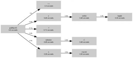
Let's take a look at the output from the profiler output for both functions

> Rprof( "goldbach5.out" ); out <- goldbach5(100000); Rprof( NULL)
> summaryRprof( "goldbach5.out" )$by.total
            total.time total.pct self.time self.pct
"goldbach5"       6.60     100.0      2.88     43.6
"<="              1.60      24.2      1.60     24.2
"+"               0.72      10.9      0.72     10.9
".C"              0.48       7.3      0.48      7.3
"unlist"          0.48       7.3      0.30      4.5
"tabulate"        0.48       7.3      0.00      0.0
"y"               0.48       7.3      0.00      0.0
"rep.int"         0.36       5.5      0.36      5.5
"x"               0.36       5.5      0.00      0.0
"lapply"          0.18       2.7      0.18      2.7
".Call"           0.08       1.2      0.08      1.2
"isprime"         0.08       1.2      0.00      0.0

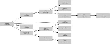
> Rprof( "goldbach4.out" ); out <- goldbach4(100000); Rprof( NULL)
> summaryRprof( "goldbach4.out" )$by.total
                 total.time total.pct self.time self.pct
"goldbach4"           31.60     100.0      1.28      4.1
"upperTriangle"       23.56      74.6      2.10      6.6
"upper.tri"           12.48      39.5      0.00      0.0
"outer"                8.98      28.4      7.38     23.4
"col"                  5.96      18.9      5.96     18.9
"row"                  5.40      17.1      5.40     17.1
"hist.default"         5.24      16.6      0.86      2.7
"hist"                 5.24      16.6      0.00      0.0
".C"                   3.98      12.6      3.98     12.6
"<="                   2.02       6.4      2.02      6.4
"FUN"                  1.60       5.1      1.60      5.1
"as.numeric"           0.54       1.7      0.54      1.7
"max"                  0.22       0.7      0.22      0.7
"seq"                  0.22       0.7      0.00      0.0
"seq.default"          0.22       0.7      0.00      0.0
"is.finite"            0.16       0.5      0.16      0.5
".Call"                0.08       0.3      0.08      0.3
"isprime"              0.08       0.3      0.00      0.0
"sort.int"             0.02       0.1      0.02      0.1
""          0.02       0.1      0.00      0.0
"median.default"       0.02       0.1      0.00      0.0
"sort"                 0.02       0.1      0.00      0.0
"sort.default"         0.02       0.1      0.00      0.0

Or a graphical display (see the R wiki for the perl script that makes the graph):

goldbach4

goldbach4.png

goldbach5

goldbach5.png

The question is now, can we go further. I believe we can, because we still allocate a lot of things we trash eventually, any takers ?

Tuesday, March 3 2009

Patching the R profiler so that it shows loops

The R profiler

The R profiler is an amazing way to find where in your code (or someone else's code) lies some inefficiency. For example, the profiler helped in this challenge on the R wiki. See also the profiling section on the http://cran.r-project.org/doc/manuals/R-exts.html#Profiling-R-code-for-speed document

What is wrong with it

The profiler, however, is not able to trace uses of loops (for, while or repeat), and consequently will not identify loops as the cause of ineffiency of the code. This is a shame, because loops in R are usually closely related to inefficiency. For example, if we profile this code:

1 Rprof( )
2 x <- numeric( )
3     for( i in 1:10000){
4       x <- c( x, rnorm(10) )
5     }
6 Rprof( NULL )
7 print( summaryRprof( ) )
8 
we get :
$ time Rscript script1.R 
$by.self
        self.time self.pct total.time total.pct
"rnorm"      0.16      100       0.16       100

$by.total
        total.time total.pct self.time self.pct
"rnorm"       0.16       100      0.16      100

$sampling.time
[1] 0.16


real	0m7.043s
user	0m5.170s
sys	0m0.675s

So the profiler only reports about 0.22 seconds, when the actual time taken is more about 5 seconds. We can show that by wrapping the entire for loop in a function:

   1 Rprof( )
   2 ffor <- function(){
   3     x <- numeric( )
   4     for( i in 1:10000){
   5       x <- c( x, rnorm(10) )
   6     }
   7 } 
   8 ffor()
   9 Rprof( NULL )
  10 print( summaryRprof( ) )
  11 

which gives this :

$ time Rscript script2.R 
$by.self
        self.time self.pct total.time total.pct
"ffor"       5.14     96.3       5.34     100.0
"rnorm"      0.20      3.7       0.20       3.7

$by.total
        total.time total.pct self.time self.pct
"ffor"        5.34     100.0      5.14     96.3
"rnorm"       0.20       3.7      0.20      3.7

$sampling.time
[1] 5.34


real	0m6.434s
user	0m5.151s
sys	0m0.698s

The ffor function takes 100 pourcent of the times, and rnorm takes only 3.7 percent of the time, instead of 100 percent, which would be the conclusion of the first example.

But in real life, it is not possible to wrap every loop in a function as this will massively break a lot of code. Instead, we could make the profiler aware of loops. This is the purpose of the patch I posted to R-devel

The details of the implementation

The patch actually only takes place in (several places of) the file eval.c

In the do_for function, a context is created for the "for" loop, using the begincontext function:

1033     begincontext(&cntxt, CTXT_LOOP, R_NilValue, rho, R_BaseEnv, R_NilValue,
1034          mkChar("[for]") );

The change here appears on the second line and simply adds a bit of information to the context that is created, similar changes are also made on the functions do_repeat and do_while.

Next, we need to grab this information at each tick of the profiler, which is the job of the doprof function:

168     if ((cptr->callflag & (CTXT_FUNCTION | CTXT_BUILTIN))
169         && TYPEOF(cptr->call) == LANGSXP) {
170         SEXP fun = CAR(cptr->call);
171         if (!newline) newline = 1;
172         fprintf(R_ProfileOutfile, "\"%s\" ",
173             TYPEOF(fun) == SYMSXP ? CHAR(PRINTNAME(fun)) :
174             "<Anonymous>");
175     } else if( (cptr->callflag & CTXT_LOOP) ){
176       if (!newline) newline = 1;
177       fprintf(R_ProfileOutfile, "\"%s\" ", CHAR(cptr->callfun) );  
178     }

The else branch will be executed when the context is a a loop context, and we just retrieve the callfun string we created in the do_for function.

Now, with this R patched, and compiled, Rprof is able to record loops

[]$ /home/romain/workspace/R-trunk/bin/Rscript script1.R
$by.self
        self.time self.pct total.time total.pct
"[for]"      5.28     97.4       5.42     100.0
"rnorm"      0.14      2.6       0.14       2.6

$by.total
        total.time total.pct self.time self.pct
"[for]"       5.42     100.0      5.28     97.4
"rnorm"       0.14       2.6      0.14      2.6

$sampling.time
[1] 5.42

[]$ head Rprof.out 
sample.interval=20000
"[for]" 
"[for]" 
"[for]" 
"rnorm" "[for]" 
"[for]" 
"[for]" 
"[for]" 
"[for]" 
"[for]"