Goldbach's Comet
By romain francois on Saturday, March 7 2009, 14:51 - Permalink
Murali Menon has posted on his blog code to calculate Goldbach partitions. Murali describes his approach to write the function, starting from brute force approach of loops, though the use of the Vectorize function, to some further optimized code using outer
This post is a follow up on Murali's attempt refining the extra mile
This is the last implementation on Murali's blog :
 1 goldbach4 <- function(n) {
 2     xx <- 1 : n
 3     xx <- xx[isprime(xx) > 0]
 4     xx <- xx[-1]
 5     z <- as.numeric(upperTriangle(outer(xx, xx, "+"),
 6                     diag = TRUE))
 7     z <- z[z <= n]
 8     hist(z, plot = FALSE,
 9          breaks = seq(4, max(z), by = 2))$counts
10 }
11
As pointed out on the blog, although this is fast thanks to the clever vectorization of outer, there is some frustration of having to allocate a matrix of size N * N when you only need the upper triangle ( N*(N+1)/2 ). Furthermore, if we look in outer, we see that not only an N*N sized vector is created for the result (robj), but also for the vectors X and Y:
31         FUN <- match.fun(FUN)
32         Y <- rep(Y, rep.int(length(X), length(Y)))
33         if (length(X))
34             X <- rep(X, times = ceiling(length(Y)/length(X)))
35         robj <- FUN(X, Y, ...)
36         dim(robj) <- c(dX, dY)
37     }
This reminded me of the fun we had a few years ago with a similar problem. See the R wiki for a detailed optimization, and I am borrowing Tony Plate's idea for the goldbach5 approach here. The idea is basically to figure out the indices of the upper triangle part of the matrix before calculating it:
12 goldbach5 <- function(n) {
13     xx <- 1 : n
14     xx <- xx[isprime(xx) > 0]
15     xx <- xx[-1]
16
17     # generates row indices
18     x <- function(N){
19         rep.int( 1:N, N:1)
20     }
21     # generates column indices
22     y <- function(N){
23         unlist( lapply( 1:N, seq.int, to = N ) )
24     }
25     z <- xx[ x(length(xx)) ] + xx[ y(length(xx)) ]
26     z <- z[z <= n]
27     tz <- tabulate(z, n )
28     tz[ tz != 0 ]
29 }
30
This gives a further boost to the execution time (only really visible with large n)
> system.time( out <- goldbach4(100000) )
   user  system elapsed
 28.268   5.389  36.347
>
> system.time( out <- goldbach5(100000) )
   user  system elapsed
  4.927   1.873   7.734
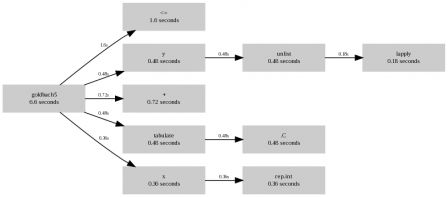
Let's take a look at the output from the profiler output for both functions
> Rprof( "goldbach5.out" ); out <- goldbach5(100000); Rprof( NULL)
> summaryRprof( "goldbach5.out" )$by.total
            total.time total.pct self.time self.pct
"goldbach5"       6.60     100.0      2.88     43.6
"<="              1.60      24.2      1.60     24.2
"+"               0.72      10.9      0.72     10.9
".C"              0.48       7.3      0.48      7.3
"unlist"          0.48       7.3      0.30      4.5
"tabulate"        0.48       7.3      0.00      0.0
"y"               0.48       7.3      0.00      0.0
"rep.int"         0.36       5.5      0.36      5.5
"x"               0.36       5.5      0.00      0.0
"lapply"          0.18       2.7      0.18      2.7
".Call"           0.08       1.2      0.08      1.2
"isprime"         0.08       1.2      0.00      0.0

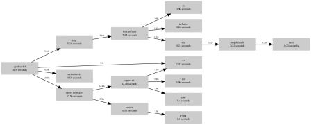
> Rprof( "goldbach4.out" ); out <- goldbach4(100000); Rprof( NULL)
> summaryRprof( "goldbach4.out" )$by.total
                 total.time total.pct self.time self.pct
"goldbach4"           31.60     100.0      1.28      4.1
"upperTriangle"       23.56      74.6      2.10      6.6
"upper.tri"           12.48      39.5      0.00      0.0
"outer"                8.98      28.4      7.38     23.4
"col"                  5.96      18.9      5.96     18.9
"row"                  5.40      17.1      5.40     17.1
"hist.default"         5.24      16.6      0.86      2.7
"hist"                 5.24      16.6      0.00      0.0
".C"                   3.98      12.6      3.98     12.6
"<="                   2.02       6.4      2.02      6.4
"FUN"                  1.60       5.1      1.60      5.1
"as.numeric"           0.54       1.7      0.54      1.7
"max"                  0.22       0.7      0.22      0.7
"seq"                  0.22       0.7      0.00      0.0
"seq.default"          0.22       0.7      0.00      0.0
"is.finite"            0.16       0.5      0.16      0.5
".Call"                0.08       0.3      0.08      0.3
"isprime"              0.08       0.3      0.00      0.0
"sort.int"             0.02       0.1      0.02      0.1
""          0.02       0.1      0.00      0.0
"median.default"       0.02       0.1      0.00      0.0
"sort"                 0.02       0.1      0.00      0.0
"sort.default"         0.02       0.1      0.00      0.0
Or a graphical display (see the R wiki for the perl script that makes the graph):
goldbach4

goldbach5

The question is now, can we go further. I believe we can, because we still allocate a lot of things we trash eventually, any takers ?
Comments
Hi Romain: thanks for the backlink and enhancements to the code. Nice work.
http://wiki.r-project.org/rwiki/dok...
404 Not Found